Position, Velocity, and Acceleration
Title: Kinematic Graphs Lab
Partner: Abbey Applegate
Date: 9/26/14
Partner: Abbey Applegate
Date: 9/26/14
Purpose
The purpose of this lab is to use two different methods to obtain the five kinematic quantities of displacement, initial velocity, time, final velocity, and acceleration of a cart rolling down a ramp. The first method involved measuring the distance and time using traditional methods, and the second method utilized a ticker tape timer and graphical analysis. Once the quantities are calculated, we will determine whether or not the cart accelerated at a constant rate.
Theory
The five fundamental kinematic quantities are defined as follows:
1. Initial velocity- velocity at the starting point
2. Displacement- object's overall change in position
3. Time- measurable period during which a process continues
4. Acceleration- rate at which an object changes its velocity
5. Final velocity- velocity at the ending point
Four kinematic equations are used to solve for the five quantities. Equation usage varies depending on the data already known or measured and the quantity missing or desired.
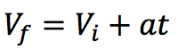
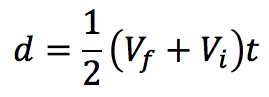
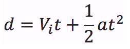
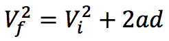
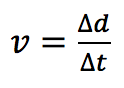
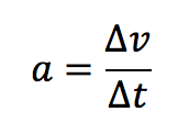
In addition, the equations for velocity and acceleration were also used to obtain data for the graphical portion of the lab.
Experimental Technique
|
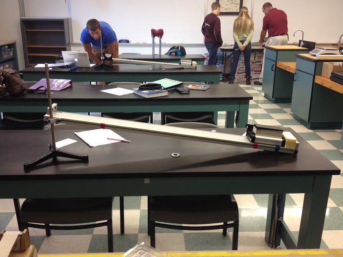
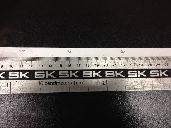
Each of the five fundamental quantities will be determined from a cart rolling down an inclined plane with an angle of 8 degrees. The apparatus was set up as shown on the right. The increment the cart was measured during was marked off using red tape, one at 25 cm and one at 100 cm.
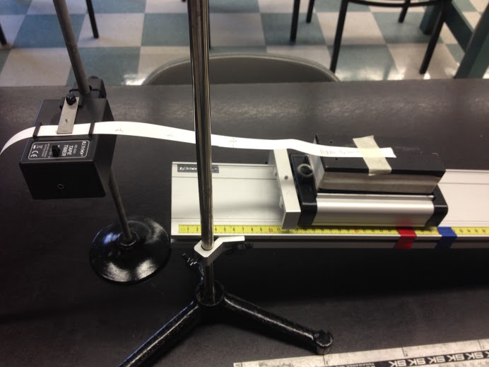
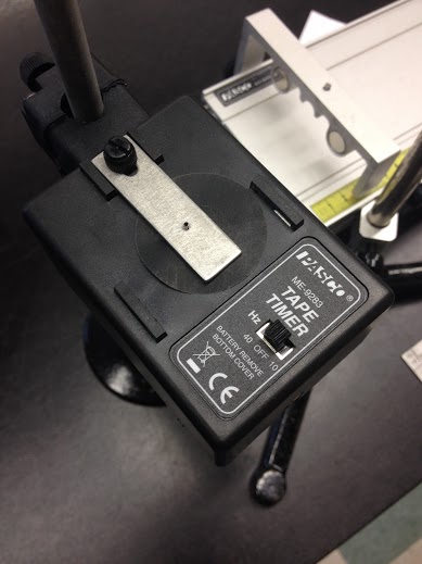
METHOD ONE- The displacement was measured using a meter stick. The time was measured using video analysis. Fundamental quantities will be determined using kinematic calculations. METHOD TWO- The device was attached to the cart as shown below and ran through to obtain data points. The displacement and time were then measured at each point. The remaining quantities will be determined using graphical analysis. |
|
Data
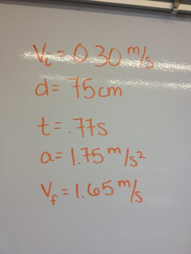
METHOD ONE- The starting point of 25 cm and the ending point of 100 cm were subtracted for a total displacement of 75 cm.
Using video analysis, 23 frames were counted, and using a conversion factor of 30 frames per second, the time was calculated to be .77 seconds.
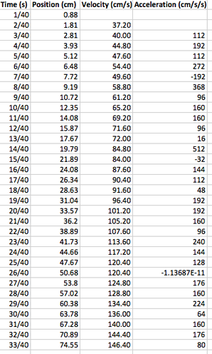
METHOD TWO- The ticker tape timer was run at 40 repetitions per second to obtain the data points shown at right.
Velocity and acceleration were calculated using the previously stated equations.
Using video analysis, 23 frames were counted, and using a conversion factor of 30 frames per second, the time was calculated to be .77 seconds.
METHOD TWO- The ticker tape timer was run at 40 repetitions per second to obtain the data points shown at right.
Velocity and acceleration were calculated using the previously stated equations.
Analysis
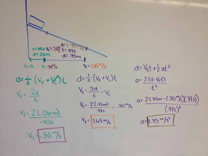
METHOD ONE- Initial velocity was calculated by finding the final velocity of the 6 cm interval preceding the experimental interval. Final velocity and acceleration were also found using kinematic equations, as shown at right.
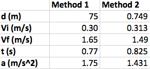
A summary of the fundamental values found using this method is shown below.
A summary of the fundamental values found using this method is shown below.
METHOD TWO- Using the data points from the ticker tape timer, which gave position and time, velocity and acceleration were calculated as shown in the data table above. Then, the following graphs were created. The five fundamental quantities were determined using the graphs.
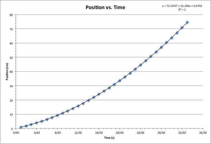
The third kinematic equation in the form of X= ½ at^2+Vit+Xi is essentially equivalent to the second order polynomial trend line that corresponds to this graph. Time can be directly read off of the graph to be 33/40 s or 0.825 s. Displacement can also be read off the graph to be 75 cm, but the initial position (third term of the equation) of 0.0702 must be subtracted to give a value of 0.749 m. Using the portion of the equation that reads ½ a and setting it equal to the value of 71.547, we can determine the acceleration to be 1.431 m/s/s. The coefficient of the second term is the initial velocity, so 31.3 cm/s or 0.313 m/s. These values can then be plugged into the first kinematic equation to give a final velocity of 1.49 m/s. Please note that the correlation coefficient is equal to 1, meaning that this data is accurate.
|
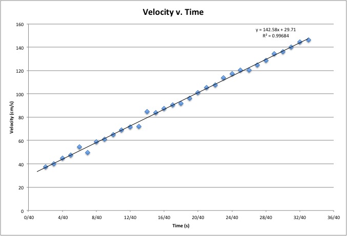
Time can once again be read off of the graph. The trend line of this graph matches the form of the first kinematic equation such that linear form y=mx+b corresponds to Vf= at + Vi. Displacement would be equal to the area under the curve, or integral, of this graph. Initial velocity is equal to the y-intercept of this equation. The acceleration is equal to the slope (tangent line) of this graph. Final velocity would need to be calculated by plugging in these values.
|
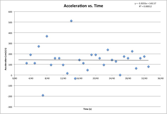
Data can be extrapolated from an acceleration versus time graph in that the area under the curve will give the velocity. However, this particular graph has a correlation coefficient of 0, so data from this graph is not reliable.
|
Conclusion
|
The purpose of this lab was to determine the five fundamental kinematic quantities using two methods: traditional hand timing and a ticker tape timer.
Sources of error for the measurements in method one include imperfect matching up of video frames and blurred images due to shutter speed. Sources of error for measurements in method two include ticker tape timer dots not aligning with the start and end points of our original incline. Bumps in the track, including tape marks, and errors in cart design could also affect the experiment. Finally, we must determine whether or not the acceleration of the car down the incline is constant. The slope of the best fit line of a velocity versus time graph represents acceleration. On our velocity versus time graph, this slope seems to be relatively constant, with a correlation coefficient of 0.99684. Thus, acceleration is constant. The slope of the velocity versus time graph is 142.58, and the best fit line of the acceleration versus time graph lies roughly in the same area, further confirming that acceleration is constant. Visible patterns are apparent, but data anomalies do exist. |
|
References
Initial Velocity. (n.d.). Retrieved October 6, 2014, from http://physics.tutorvista.com/motion/initial-velocity.html
Distance and Displacement. (n.d.). Retrieved October 6, 2014, from http://www.physicsclassroom.com/class/1DKin/Lesson-1/Distance-and-Displacement
Time. (n.d.). Retrieved October 6, 2014, from http://www.merriam-webster.com/dictionary/time
Acceleration. (n.d.). Retrieved October 6, 2014, from http://www.physicsclassroom.com/class/1DKin/Lesson-1/Acceleration
Final velocity. (n.d.). Retrieved October 6, 2014, from http://physics.tutorvista.com/motion/final-velocity.html
Giancoli, D. (1998). Physics: Principles with Applications (5th ed.). Upper Saddle River, N.J.: Prentice Hall.
Lahs Physics (n.d.). Retrieved October 6, 2014, from www.lahsphysics.weebly.com
